I had a math modelling assignment a while ago that required us to simulate the spread of rumors within a social media network. I ended up choosing Twitter, as its content is the most straightforward. My goal was to set up a system that could predict the likelihood of a retweet on a per user basis, and to arrange all of those predictions into a graph that could simulate the spread of a retweet throughout the network. I ended up using a Naive Bayes Classifier to accomplish this. The math behind it is quite approachable, and it’s currently used in a number of different applications despite its naive assumptions. This post will describe how it works, and give a sense of how it might be improved in the future. If you want to fast forward and check it out, it’s hosted here.
Step 1: Ingest Relevant Tweets
In order to predict what a given user will or will not retweet, we want a history of all of the tweets that they might have seen. Some of these tweets will be classified as positive (retweeted), and the rest will be classified as negative (not retweeted). Assuming users only see tweets from people they follow, I downloaded all of the tweets from each of the users a user in our network was following.
There are a number of issues with this approach. First, we don’t know whether or not those tweets were actually seen by the user. They might not have been online, or never made it to that retweet on their timeline, but our model doesn’t know that and will penalize content that our user may have retweeted had they actually seen it. Second, there may be users that were previously followed and then unfollowed, which will not make it into our pool/not give us a full picture of our user’s history. Third, we are assuming that a user’s tastes are relatively constant, and that the content is more important than other factors that might influence their retweet (what they were doing, what time of day it was, what other people were retweeting, what kind of mood they were in, how old they were at the time, etc).
If we wanted to improve our model, we could improve our pool and add some of the other factors we described.
Step 2: Analyze Tweets
The first step with any sort of text analysis is to tokenize the text being analyzed. Tokenizing just means breaking down a long string into smaller pieces. A common way to tokenize text is to break it into individual words. This is what I did via nltk’s Tweet Tokenizer. There’s a bit of extra sugar in there (removes handles, removes repeated characters, removes html), but all we need to know is that it’s breaking down the tweet into words. More sophisticated text analysis often makes use of N-Grams, which are groups of tokens, but for our bare bones, very simple model, we only care about individual tokens.
Bayes’ Theorem is all about calculating probabilities based on observation. So all that we need to do during our analysis is count occurrences; we want to count the occurrences of tokens that were in tweets that were retweeted, and count the occurrences in tweets that were not retweeted. For example, consider the tweet “I am a cool guy”, which was retweeted, and “I think cars are cool”, which was not retweeted. The occurrences of each token will be as follows:
{
  words: {
    a: {
      negative: 0,
      positive: 1
    },
    am: {
      negative: 0,
      positive: 1
    },
    are: {
      negative: 1,
      positive: 0
    },
    cars: {
      negative: 1,
      positive: 0
    },
    cool: {
      negative: 1,
      positive: 1
    },
    guy: {
      negative: 0,
      positive: 1
    },
    think: {
      negative: 1,
      positive: 0
    },
    I: {
      negative: 1,
      positive: 1
    },
  },
  total_positive: 5,
  total_negative: 5
}
Once we’ve gone through all of the tweets, we’ll have a large set of tokens per user with counts of negative and positive occurrences for each individual token, along with total token occurrence counts.
Step 3: Predict Retweets
Now we have all the pieces we need in order to classify a new tweet as something retweeted or not retweeted. Let’s say the tweet we want to simulate is “cool beans”.
Our Naive Bayes Classifier will work by describing two classes: retweeted and not retweeted. Each class is applied on a per token basis. The applied version of Bayes’ Theorem we will use is as follows, where “x” is our token, and “Ck” is our class:
First, we’ll look at the positive class for a given token; let’s say “cool”. Our use of the equation then reads: “The probability of a tweet being retweeted given it has the word ‘cool’ is equal to the observed probability of a tweet being retweeted times the observed probability of ‘cool’ being in a retweeted tweet divided by the probability of ‘cool’ appearing in any tweet”.
To determine the probability of the class as a whole, we add up all the occurrences of tokens that were in any tweet that was retweeted, and divide it by the total number of tokens in all the tweets. Let’s say there were 10,000 tokens in total, that there were 1,000 token occurrences in retweets and 9,000 token occurrences in tweets that were not retweeted. That means our “p(Ck)” is 1,000/10,000, or .1
Let’s say that after we look at all the tweets a given user has looked at, the token “cool” appears 10 times in tweets that were retweeted and 40 times in tweets that were not retweeted. That means the observed probability for our particular token being in a retweeted tweet, or “p(x|Ck)” is 10/1,000, or .01
Now all that’s left is “p(x)”, which in this case would be 50/10,000 (total times token “cool” appeared over total times all tokens appeared), or .005
If we plug those numbers into our equation, we get (.1 · .01)/(.005) = .2
Let’s say we’re lucky and that “beans” has the same exact probabilities as “cool”. All we need to do to find the classifier value for the whole tweet is to multiply each of the probabilities for the same class together, so the value for the positive classification for the tweet “cool beans” would be .2 · .2 = .04
This does NOT mean that the probability of the tweet being retweeted is .04, however. We can see that by calculating the negative classifier. In that case, p(x) would stay the same, at .005, p(Ck) would change to 9,000/10,000 or .9, and p(x|Ck) would change to 40/9,000 or ~.004444. Our equation for “cool” being in a negative tweet would then be (.9 · .004444)/(.005) ~= .8, which is the same for “beans”, which means the negative classification for “cool beans” would be .8 · .8 = .64 . This does not add up with our positive classification of .04 to 1.
Normally, we’d just classify the tweet as whatever the greatest classifier value is. So in the case of “cool beans”, the tweet would be classified as “Not Retweeted” (bummer). However, since most tweets users see are not retweeted, we’d have a simulation that would classify most tweets as not being retweeted. In order to add some realism, the final simulation has a “non deterministic” mode that uses the negative and positive classifier values to come up with a probability of being retweeted. In the case of “cool beans”, this value would be .04 / (.04 + .64) ~= .05882 . So although this tweet will normally not be retweeted, there’s still a chance of a retweet occurring if you run the simulation enough times.
Step 4: Results
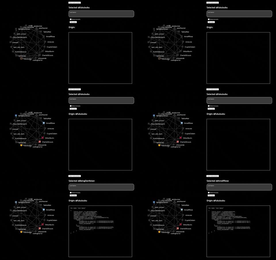
The realism of this model is dubious, considering our extremely naive algorithm, our naive tokenization, and the naive assumptions we made when collecting our data. However, a couple sample tweets seemed to be given reasonable looking retweet chances based on the network (which is primarily people interested in new technology), so it may work.